First order mass fraction and temperature

From (8.17), (8.27) and (8.45),

$$A_{m1} \equiv \mbox{\textit{Sc}}\;\mathbf{u}_0\cdot\mbox{\boldmath$\nabla$}m_0$$

$$= \mbox{\textit{Sc}}\;\frac{r}{80}\left(1-4r^2\right)\sin\theta\,\mbox{\boldmath$\hat{\phi}$}\cdot \mbox{\boldmath$\nabla$}(r\sin\theta\cos\phi)$$

$$= -\mbox{\textit{Sc}}\;\frac{r}{80}\left(1-4r^2\right)\sin\theta\sin\phi$$

$$= -\mbox{\textit{Sc}}\;\frac{r}{80}\left(1-4r^2\right)P_1^1(\cos\theta)\sin\phi.$$ (8.48)

The solution for (8.14) for $i=1$ is then:

$$m_1 = \frac{\mbox{\textit{Sc}}}{44\,800}r(1-4r^2)(9-20r^2)\sin\theta\sin\phi.$$ (8.49)

Similarly,

$$T_1 = \frac{\mbox{\textit{Pr}}}{44\,800}r(1-4r^2)(9-20r^2)\sin\theta\sin\phi.$$ (8.50)

Noting that $y=r\sin\theta\sin\phi$, and $r^2=x^2+y^2+z^2$, it can be seen that $m_1$ depends on the Cartesian coordinates only as $m_1=m_1(y,x^2+z^2)$, so that it is axisymmetric about the $y$-axis. Its contours in any plane passing through the $y$-axis are plotted in figure 8.5;

Figure 8.5: First order vapour mass fraction (8.49) or temperature (8.50) in any plane passing through the $y$-axis. $m_1$ and $T_1$ are nonnegative for $y\geq 0$. Contour levels at 0.01, 0.1(0.1)0.4, 0.6(0.1)0.9, 0.99 of range.

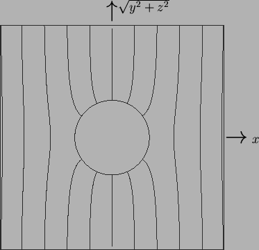it is nonnegative in the upper hemisphere, $0\leq\phi\leq\pi$.

The vapour mass fraction field to first order, $m_0+\mbox{\textit{Gr}}(1+N)m_1$, is contoured for various values of $\mbox{\textit{Gr}}(1+N)\mbox{\textit{Sc}}$ in figure 8.6.

Figure 8.6: Vapour mass fraction in the plane $z=0$ to first order, $m_0+\mbox{\textit{Gr}}(1+N)m_1$, for $\mbox{\textit{Gr}}(1+N)\mbox{\textit{Sc}}$ of (a) 500, (b) 1000, (c) 2000, (d) 5000, (e) 10000, (f) 13000. Contours at $m=-0.4(0.1)0.4$.

The contours could also be interpreted as the temperature, $T_0+\mbox{\textit{Gr}}(1+N)$, for the corresponding value of $\mbox{\textit{Gr}}(1+N)\mbox{\textit{Pr}}$. By $\mbox{\textit{Gr}}(1+N)\mbox{\textit{Sc}}=$13000, the mass fraction field has begun to exhibit internal extrema, which is impossible for the full solution, $m$, by Theorem 1. Since $m\sim m_0+\mbox{\textit{Gr}}(1+N)m_1$, the plots should be increasingly accurate for the lower values of $\mbox{\textit{Gr}}(1+N)$; comparison with higher order approximations or full solutions would be required to quantify this. Some of the qualitative features of convection in plane vertical cavities, for example as seen in figure 5.8, are evident in figure 8.6, even at this low order: the stretching of the level curves at the departure `corners', meaning the quadrants $xy>0$; steepening of the horizontal gradients at the starting `corners', $xy<0$; and the beginnings of a stable vertical stratification in the core.

In comparing the present results with those for vertical plane rectangular cavities (ch. 5), it may be seen that the `destruction of the conduction-diffusion regime by a gradual penetration of convective effects into the core' (p. ) occurs at any finite value of $\mbox{\textit{Gr}}(1+N)\mbox{\textit{Sc}}$ or $\mbox{\textit{Gr}}(1+N)\mbox{\textit{Pr}}$ in the sphere. This is because the `end-zones' of the spherical enclosure are simply the upper and lower hemispheres: nowhere is `sufficiently far from the floor or ceiling' (p. ).

The behaviour outside the plane $z=0$ can easily be visualized by noting that to first order, $m\sim x+O(\mbox{\textit{Gr}}^2)$ in the plane $y=0$, while in the plane $x=0$, $m_0=0$, so that $m\sim m_1+O(\mbox{\textit{Gr}}^2)$, which is pictured in figure 8.5.