The conduction-diffusion regime

That the temperature and mass fraction are practically independent of height near $y=\mbox{$\mathcal A$}/2$ in the examples of figure 5.8 is qualitatively evident. To quantify the extent of the fully developed region, and hence the existence or otherwise of the conduction-diffusion regime, the discrepancies between the finite element solution and the fully developed profiles (4.24)-(4.26), now subscripted with $\infty$, are introduced:

$$m' = m - m_{\infty};$$ (5.7)

$$u' = \frac{u-u_{\infty}}{\max \vert u\vert};$$ (5.8)

$$v' = \frac{v-v_{\infty}}{\max \vert v\vert};$$ (5.9)

$$\frac{\partial p'}{\partial y} = \frac{\frac{\partial p}{\partial y}-\frac{\,\mathrm{d}p_{\infty}}{\,\mathrm{d}y}} {\frac{\,\mathrm{d}p_{\infty}}{\,\mathrm{d}y}};$$ (5.10)

$$T' = T - T_{\infty}.$$ (5.11)

The maxima in the definitions of the velocity component discrepancies, $u'$ (5.8) and $v'$ (5.9) are taken over the nodal values of the Fastflo solution.

Determination of the velocity profile, $v_{\infty}$, from (4.27), requires evaluation of the integration constant $c$. Here, $c$ was chosen so as to minimize the root-mean-square discrepancy on the mid-height line, $y=\mbox{$\mathcal A$}/2$, using the 32 nodal values. This value of $c$ can then be checked against the numerical vertical pressure gradient via (4.28) and (5.10). Figure 5.9 plots the discrepancies for the same run as

Figure 5.9: Discrepancies between the Fastflo and analytic solutions: (a) $u'$, (b) $v'$, (c) $T'$, (d) $m'$ and (e) $\partial p'/\partial y$. Same run as figures 5.8(d-f). Contours shown at $\pm1,2$ and 5%, with signs marked by circled symbols.

figures 5.8(d-f).

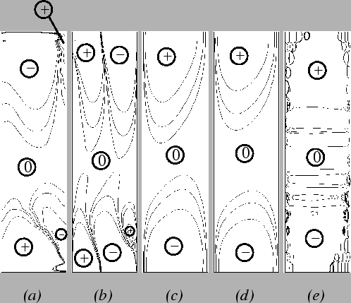The obvious irregularity of the pressure field in figure 5.9(e) is not unexpected, nor is it necessarily of purely numerical origin. Pressure singularities were anticipated in the corners due to the multivalued boundary condition on $u$ (§3.3.3). They do appear to have deleteriously affected large regions of the pressure solution, but the result in the fully developed zone accords with the analytic solution of chapter 4.

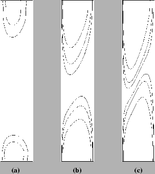
Since the discrepancies (5.7)-(5.11) are less than 1% for some continuous horizontal lines in each of figures 5.9(a-e), this set of parameters pertains to the conduction-diffusion regime. The proportion of the height of the cavity between the end-zones is small, so that this case is near the limit of the regime. To investigate this, Fastflo solutions were obtained for the same set of parameters except for the vertical aspect ratio, $\mathcal A$, which was varied. The temperature discrepancy, $T'$, is plotted in figure 5.10. These plots clearly reveal that the

Figure: The effect of $\mathcal A$ on the existence of the conduction-diffusion regime. Temperature discrepancy levels as in figure 5.9(c). $\mbox{\textit{Gr}},\,\mbox{\textit{Sc}},\,\mbox{\textit{Pr}}_r,\,\mbox{\textit{Pr}}_I,\,N$ and $\varPhi$ as in figures 5.8(d-f).

conduction-diffusion regime can be destroyed simply by decreasing the vertical aspect ratio--the critical aspect ratio here being somewhere between 2 and 5. The idea, then, that the boundary of the regime could depend simply on a critical combined Grashof or Rayleigh number (based on the cavity width) is false. Another interesting feature of figure 5.10 is the similarity of the end-zones in the cavities of vertical aspect ratio 5 and 10. This suggests that it may be possible to correlate the overall energy transfer rates in a form analogous to that proposed by Batchelor (1954; see also Lee & Korpela 1983) for the conduction regime in the pure fluid problem:

$$\mbox{$\mathcal A$}\overline{\mbox{\textit{Nu}}} = \mbox{$\m... ...tit{Sc}},\mbox{\textit{Pr}}_r,\mbox{\textit{Pr}}_I,N,\varPhi )$$ (5.12)

where $\mbox{\textit{Nu}}$ is a dimensionless energy transfer rate and the overbar denotes an average over $0<y<\mbox{$\mathcal A$}$. The complete set of average sensible Nusselt numbers from the Fastflo runs is given in table 5.3.

Table: Sensible Nusselt numbers, $\mbox{\textit{Nu}}_{sen}$, from Fastflo runs for $\varPhi =0.69, N=0.5, \mbox{\textit{Pr}}_r=0.71, \mbox{\textit{Pr}}_I=\mbox{\textit{Sc}}=0.61$.

	$\mathcal A$
$\mbox{\textit{Gr}}(1+N)\mbox{\textit{Pr}}_r$	2	5	10
100	1.00	1.00	1.00
1000	1.17	1.08	1.04
2000	--	1.08	1.11
5000	--	--	1.32

This validity of this approach was demonstrated in an earlier joint paper (McBain & Harris 1998, fig. 6), using the data of table 5.3 and Dr Harris's FIDAP solutions.

A similar result may be expected to hold for the overall mass transfer rate.

The other principal parameter involved in the determination of the conduction-diffusion regime is the combined Grashof number, $\mbox{\textit{Gr}}(1+N)$. Figure 5.11 shows how the regime can be

Figure 5.11: Destruction of the conduction-diffusion regime by a gradual penetration of convective effects into the core as the Grashof number increases. $\mbox{\textit{Gr}}(1+N)\mbox{\textit{Pr}}_r=$ (a) 100, (b) 1000 and (c) 2000. Temperature discrepancy contours, levels as in figure 5.9(c). $\mbox{\textit{Sc}}, \mbox{\textit{Pr}}_r, \mbox{\textit{Pr}}_I, N, \mbox{$\mathcal A$}$ and $\varPhi$ as in figures 5.8(d-f).

destroyed by increasing Gr with all other parameters fixed.