It may be worthwhile at the outset to note that although low Reynolds number expansions for unbounded domains, e.g. viscous flow past a solid sphere (Lamb 1932, p. 609; Van Dyke 1964, ch. 8), are singular perturbation problems, this is not the case for bounded domains (Munson & Joseph 1971). This makes sense: the region of nonuniformity in the former class of problems, where the neglected inertial terms are not negligible in comparison to the retained viscous terms, is typically a neighbourhood of the point at infinity.
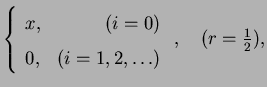
Assume asymptotic expansions for the vapour mass fraction, velocity,
pressure and temperature of the form:
| (8.10) | |||
| (8.11) | |||
| (8.12) | |||
| (8.13) |
Substituting these in to the low mass transfer rate equations,
(6.16)-(6.19), and taking the limit
![]() leads to a hierarchy of problems:
leads to a hierarchy of problems:
| (8.19) | |||
| (8.20) | |||
| (8.21) |
The series for ![]() ,
, ![]() and
and
![]() are to be taken as zero if the lower index (zero) exceeds the upper;
i.e. when
are to be taken as zero if the lower index (zero) exceeds the upper;
i.e. when ![]() . Each
. Each ![]() and
and ![]() satisfies a Laplace or Poisson equation, with source given in terms of
previously calculated quantities. These are, in principle, all soluble by
expanding the source term and the independent variable in spherical harmonics.
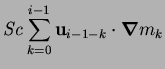
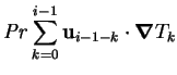
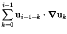
For the equations of motion, however, the presence of the
unknown pressure terms and the continuity constraints means that at each
order a Stokes problem with known `body force' must be solved.
The Stokes problem in a sphere
can be reduced to an uncoupled unconstrained set of scalar partial
differential equations (Poisson and inhomogeneous biharmonic equations) by
decomposing the velocity term into its poloidal and toroidal parts. This
technique is summarized in appendix B.
satisfies a Laplace or Poisson equation, with source given in terms of
previously calculated quantities. These are, in principle, all soluble by
expanding the source term and the independent variable in spherical harmonics.
For the equations of motion, however, the presence of the
unknown pressure terms and the continuity constraints means that at each
order a Stokes problem with known `body force' must be solved.
The Stokes problem in a sphere
can be reduced to an uncoupled unconstrained set of scalar partial
differential equations (Poisson and inhomogeneous biharmonic equations) by
decomposing the velocity term into its poloidal and toroidal parts. This
technique is summarized in appendix B.
The evaluation of ![]() may be tedious, but can be simplified by
noting that except for
may be tedious, but can be simplified by
noting that except for ![]() the terms of the series occur in pairs:
the terms of the series occur in pairs:
| (8.24) |
| (8.25) |