Elliptic section

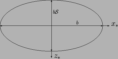
For elliptic sections, with one axis of length $b$ parallel to the $x$-axis and the other of length $\mbox{$\mathcal S$}b$ parallel to the $z$-axis, the domain is again given by (7.60) (see fig. 7.5).

Figure 7.5: Geometry for elliptic sections.

The forced flow solution (Lamb 1932, p. 587), is

$$\frac{v_f\!\!\raisebox{1ex}{\scalebox{1.414}[0.7071]{$\circ$... ...rm{d}Y} = \frac{1-4(X^2+Z^2)}{8(1+\mbox{$\mathcal S$}^{-2})}$$ (7.66)

Although equation (7.20) could be solved for $\Omega\raisebox{1ex}{\scalebox{1.414}[0.7071]{$\circ$}}$ by using the Jones-Furry solution (7.24) as a particular integral and the inverse hyperbolic cosine conformal mapping (Carslaw & Jaeger 1959, pp. 439-40), a possible form for the solution is suggested by those in $\Omega^{\parallel}=\{\mathbf{X}:X^2<1/4\}$, equation (7.24), and $\Omega\raisebox{1ex}{$\circ$}$, equation (7.65):

$$v_n\!\!\raisebox{1ex}{\scalebox{1.414}[0.7071]{$\circ$}}(X,Z) \stackrel{?}{=} \frac{X[1-4(X^2+Z^2)]}{g(\mbox{$\mathcal S$})}.$$ (7.67)

This certainly satisfies the boundary condition (7.1) on $\upartial \Omega\raisebox{1ex}{\scalebox{1.414}[0.7071]{$\circ$}}$, and it also satisfies (7.20) on $\Omega\raisebox{1ex}{\scalebox{1.414}[0.7071]{$\circ$}}$ if $g(\mbox{$\mathcal S$})=8(3+\mbox{$\mathcal S$}^{-2})$. Thus

$$v_n\!\!\raisebox{1ex}{\scalebox{1.414}[0.7071]{$\circ$}}(X,Z) = \frac{X[1-4(X^2+Z^2)]}{8(3+\mbox{$\mathcal S$}^{-2})}.$$ (7.68)

Contours of the vertical component of velocity due to buoyancy, $v_n\!\!\raisebox{1ex}{\scalebox{1.414}[0.7071]{$\circ$}}$, are displayed for elliptic sections of various spanwise aspect ratio in figure 7.6.

Figure 7.6: Fully developed buoyancy-induced flow in various elliptic sections. Curves can be interpreted as either vortex-lines or contours of the vertical component of velocity with levels at $\pm20, 40, 60$ and $80\%$ of maximum. $\oplus$ and $\ominus$ mark extrema of $v_n$ (points of zero vorticity).

Again, the curves can alternatively be interpreted as vortex-lines.

Notice that the solution for the circular cylinder (7.65) is regained for $\mbox{$\mathcal S$}=1$, while

$$v_n\!\!\raisebox{1ex}{\scalebox{1.414}[0.7071]{$\circ$}}\sim... ...) \qquad(\mbox{$\mathcal S$}\rightarrow\infty, Z\rightarrow 0)$$ (7.69)

and

$$v_n\!\!\raisebox{1ex}{\scalebox{1.414}[0.7071]{$\circ$}}\sim... ...^2) \qquad(\mbox{$\mathcal S$}\rightarrow 0, X\rightarrow 0).$$ (7.70)

Thus, $v_n\!\!\raisebox{1ex}{\scalebox{1.414}[0.7071]{$\circ$}}$ includes the Jones-Furry (7.24) and Hele-Shaw (7.27) limits as special cases, as does the solution for the rectangular domain.

Apart from the simplicity of the result (7.68), the elliptic section is remarkable for two reasons. First, the velocity profile in the plane $Z=0$ has the same odd-symmetric cubic shape as the Jones-Furry flow (7.24) for all values of $\mathcal S$; only the amplitude varies. The second is the comparative ease with which the thermal boundary conditions (7.2) may be imposed. Consider the cavity or duct to be surrounded by a highly conducting solid in which, at large distances, the temperature gradient is uniform and parallel to the $x$-axis. The problem of the temperature distribution in the solid is analogous to that for potential flow relative to an elliptic cylinder moving uniformly along the axis. From the solution to the latter problem (Lamb 1932, p. 84), it can be seen that the temperature at the section boundary varies linearly with $x$; i.e. (7.2) applies with $I=0$. If the vapour mass fraction exerted by the boundaries is a function of temperature, and $\Delta T_*$ is small enough for this to be linearized, then the same applies to the boundary conditions on $m$ (7.5).