Postprocessing

The solution variables are not always those most suitable for presentation, and they may not be the ones of interest. The velocity vector plot (fig. 5.4a), for example, is very cluttered. The temperature contour plot (fig. 5.4b) suggests that the heat transfer is practically one-dimensional throughout much of the height of the cavity, with deviations only near the horizontal surfaces. It is difficult, though, to quantify this from the figure.

The flow field is more readily envisaged with stream-lines. These are easily generated in Fasttalk (CSIRO 1997, p. 121) and are plotted in figure 5.5(a).

The question of whether or not the

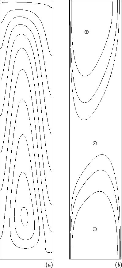
Figure 5.5: Processed solution variables from the same run as figure 5.4: (a) stream-function, with contours at $1, 10, 20,\ldots, 90, 99\%$; (b) temperature discrepancy, $T'$, with contours at $\pm1,2$ and 5%, with signs as shown.

temperature profiles are fully developed is easily answered by subtracting the finite element solution from the analytic solution, for a cavity of infinite vertical aspect ratio, equation (4.26), and contouring the result, $T'$. Figure 5.5(b) clearly displays the range of influence of the horizontal surfaces into the cavity core. This question is taken up in more detail in §5.5.

Further insight into the energy transfer can be obtained from vector plots of each of the component energy fluxes, defined by (2.48)-(2.51). It must be noted that this separation of $\mathbf{e}$ into its component parts is not unique, since it suffers from the same arbitrariness (an additive constant without physical significance) as the thermodynamic internal energy (Guggenheim 1959, p. 11). The present choice is convenient as it means that both the advective, $\mathbf{e}_{adv}$ (2.49), and interdiffusive, $\mathbf{e}_{int}$ (2.50), fluxes vanish at the left wall, since these are proportional to the reduced temperature, $T$. This simplifies calculation of the overall energy transfer rate, which thus can be accomplished by integrating just the conduction, $\mathbf{e}_{cond}$ (2.48), and latent, $\mathbf{e}_{lat}$ (2.51), parts over the cold wall. Alternatively, the total energy flux can be integrated over the domain. The conductive, advective and interdiffusive fluxes are plotted in figure 5.6.

Figure 5.6: Energy flux components: (a) conduction, $\mathbf{e}_{cond}$; (b) bulk advection, $\mathbf{e}_{adv}$; and (c) interdiffusion, $\mathbf{e}_{int}$. Arrows scaled to the maximum magnitude of each component.

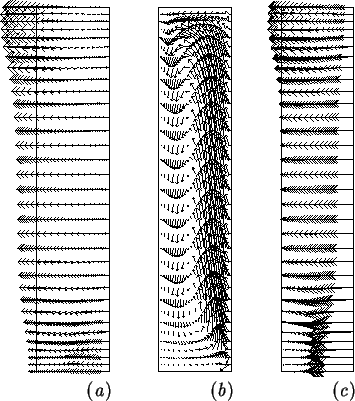The component fluxes, $\mathbf{e}_{cond}$, $\mathbf{e}_{adv}$ and $\mathbf{e}_{int}$, unlike their sum, $\mathbf{e}$, are not solenoidal. Figure 5.6 shows how the energy is transported into the cavity from the right wall by advection and interdiffusion, how these fluxes are converted to the conduction flux, and finally how energy is conducted out of the cavity into the left wall. The arrows in figure 5.6(c) which seem to be leaving the cavity in fact are not; this is another example of the cluttered nature of vector plots which is treated by the `heat-lines' introduced below.

The total energy flux is obtained from the component fluxes and (2.47) and is plotted in figure 5.7(a).

Figure 5.7: Energy transfer in the cavity: (a) energy flux vector, $\mathbf{e}$, and (b) `heat-lines'.

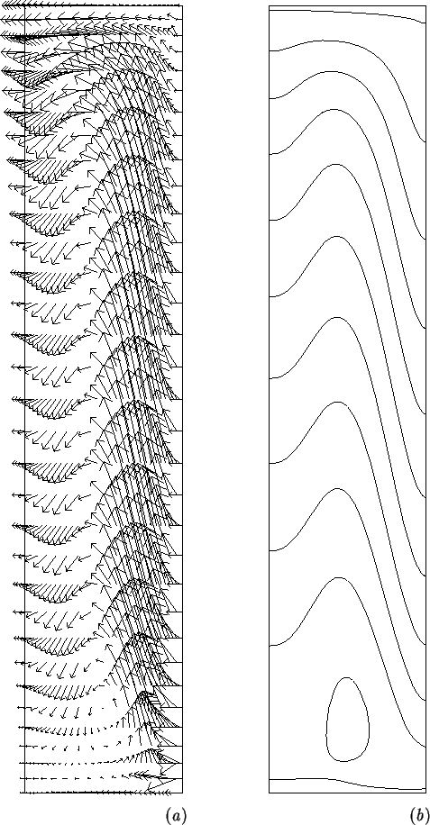Since the energy flux vector, $\mathbf{e}$, like the velocity, $\mathbf{u}$, is plane and solenoidal, a `heat-function' can be formed by analogy with the stream-function (Trevisan & Bejan 1987), and is easily implemented in Fasttalk. In fact, the same Fastflo `problem' can be used for the stream-function as the heat-function; it is merely a matter of passing either the velocity field, $\mathbf{u}$, or the energy flux field, $\mathbf{e}$. The heat-lines, the contours of the heat-function (fig. 5.7b), show the paths that energy follows through the cavity, though it is affected by the arbitrariness of the energy flux vector. Since an equal amount of energy flows between each of the heat-lines, it is clear from figure 5.7(b) that the local flux through the left wall is strongest nearer the top, and decreases down the wall. This comes about because hot vapour-rich air is convected across the top of the cavity by the counterclockwise rotating cell visible in the stream-line plot (fig. 5.5a).