Overall transfer rates

The overall energy transfer rates may be calculated from (2.66) or by averaging the horizontal component of the total energy flux (2.47) over any vertical line segment joining the floor and the ceiling (since these boundaries are adiabatic). The latter is chosen here as a test of the overall conservation of energy and the accuracy of the postprocessing operations involved in the calculation of $e$. Results are presented for averages over the left wall, the right wall and the total domain in Table 5.2.

Table 5.2: Overall energy transfer rate and test of conservation of energy.

$\mbox{$\mathcal A$}^{-1}\int_{0}^{\mathcal{A}} e\vert _{x=0} \,\mathrm{d}y$	1.0788
$\mbox{$\mathcal A$}^{-1}\int_{0}^{\mathcal{A}} e\vert _{x=1} \,\mathrm{d}y$	1.0800
$\mbox{$\mathcal A$}^{-1}\int_{0}^{\mathcal{A}}\!\!\int_{0}^{1} e\,\,\mathrm{d}x\,\,\mathrm{d}y$	1.0843

As can be seen, the estimates of the overall energy transfer rate agree with each other to within 0.5%.

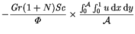
The postprocessing for the mass transfer is similar to that for the energy transfer. The details are omitted, though the overall transfer rate can be inferred from equation (2.62) and table 5.1:

$$\overline{\mbox{\textit{Sh}}} = -\frac{\mbox{\textit{Gr}}(1+N)\mbox{\textit{Sc}}}{\varPhi }\times... ...\int_0^{\mathcal{A}}\int_0^1 u \,\mathrm{d}x\,\mathrm{d}y}{\mbox{$\mathcal A$}}$$

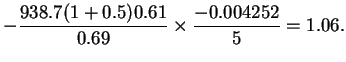$$= -\frac{938.7(1+0.5)0.61}{0.69}\times\frac{-0.004252}{5} = 1.06.$$ (5.6)

The closeness of the average transfer rates to unity is indicative of both the aptness of the scales chosen in §2.3.4 and the low degree of convective enhancement with the present parameter values.