Geometry

In order to solve the system of equations developed above, a domain and boundary conditions must be specified. Various limiting cases of the vertical cuboid are considered in chapters 4-7.

One opposing vertical pair of walls are taken to be the source and sink of vapour, while the other four walls, the front, back, floor and ceiling, serve mainly to bound the domain. Let uniform temperatures and vapour mass fractions be specified on the hot ($T=m=1$) and cold ($T=m=0$) walls, and take the others to be impermeable, postponing the question of their thermal boundary conditions. The cuboid is defined by one length scale, $b$, which is taken to be the distance separating the hot and cold walls, and two aspect ratios: $\mathcal A$, vertical; and $\mathcal S$, spanwise. As illustrated in figure 2.1,

Figure 2.1: Cuboid domain geometry, in (a) primitive and (b) normalized coordinates. The gravitational field strength is also shown in (a).

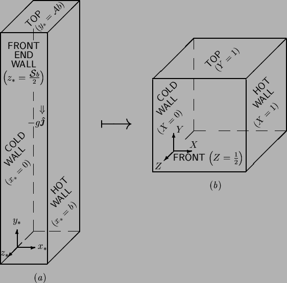the cold and hot walls lie in the planes $x=0$ and 1, respectively; the $y$-axis is vertical and the $z$-axis is chosen so as to form a right-handed system with $x$ and $y$. Since solutions of (2.52)-(2.55) are symmetrical about the central spanwise plane--the corresponding result for the analogous single fluid heat transfer problem was stated and used by Mallinson and de Vahl Davis (1977)--the origin of the coordinate system is located halfway along the base of the cold wall. Note that the centrosymmetry properties of the analogous single fluid heat transfer problem (see §2.4) described by Gill (1966) do not hold for the solutions of the present system.

In addition to the simply nondimensionalized coordinates:

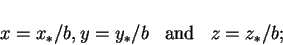$$x=x_*/b, y=y_*/b\;\;\;\mbox{and}\;\;\; z=z_*/b;$$ (2.73)

the a normalized set

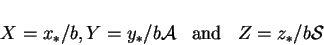$$X=x_*/b, Y=y_*/b\mbox{$\mathcal A$}\;\;\;\mbox{and}\;\;\; Z=z_*/b\mbox{$\mathcal S$}$$ (2.74)

is also useful. The transformation from primitive to normalized coordinates, in which the cuboid becomes a unit cube, is illustrated in figure 2.1. The normalized coordinates have the advantage of having a unit range. The apparent disadvantage that the expression for nabla in terms of them is more cumbersome;

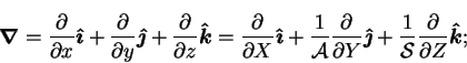$$\mbox{\boldmath$\nabla$}= \frac{\partial }{\partial x}\mbox{... ...cal S$}}\frac{\partial }{\partial Z}\mbox{\boldmath$\hat{k}$};$$ (2.75)

is in fact also an advantage, since it moves the parameters $\mathcal A$ and $\mathcal S$ from the boundary conditions to the field equations. Great use will be made of this in examining limiting forms of the cuboid in chapters 4 and 7.