The Stokes problem in the sphere

I present here a general solution of the inhomogeneous Stokes problem in the sphere with unit diameter.

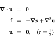
The general solution for the case $\mathbf{f=0}$, but with inhomogeneous boundary conditions has been discussed by Palaniappan et al. (1992) and Padmavathi et al. (1998).

An identity that will be used frequently is:

$$(\mbox{\boldmath$\nabla$}\times)^3(\mathbf{r}s) = -\mbox{\boldmath$\nabla$}\times(\mathbf{r}\nabla^2s)$$ (B.18)

for any scalar $s$ (Moffatt 1978, p. 19).

Lemma 3 (Zero vector fields)   If a vector field, $\mathbf{v}$, is both solenoidal and irrotational in a simply connected domain and has zero normal component over the surface, then $\mathbf{v}$ vanishes identically in the domain.

Proof: The lemma is elementary; its proof is contained in most texts on vector analysis, potential theory or continuum mechanics--see, for example, Lamb (1932, pp. 37-41).

Basically, the irrotationality implies that the field may be expressed as the gradient of a scalar, the solenoidality implies that the scalar is harmonic and the boundary conditions imply that the scalar is uniform.$\Box$

Theorem 4 (Creeping flow in a sphere)   If $\mathbf{f}$ is a vector field with Hölder continuous second order partial derivatives in the sphere $\{0\leq r\leq \mbox{$\frac{1}{2}$}\}$, then the solution of the inhomogeneous Stokes problem,

$$\begin{eqnarray*} \mbox{\boldmath$\nabla$}\cdot \mathbf{u} & = & 0 \\ \mathbf{f... ...u} \\ \mathbf{u} & = & \mathbf{0},\quad(r=\mbox{$\frac{1}{2}$}) \end{eqnarray*}$$

is

$$\begin{eqnarray*} \mathbf{u} & = & (\mbox{\boldmath$\nabla$}\times)^2(\mbox{$\ma... ...= & -\mbox{$\mathcal S$}[\mathbf{f}] - s + \mbox{\rm a constant} \end{eqnarray*}$$

where $\mbox{$\mathcal P$}[\mathbf{u}]$, $\mbox{$\mathcal T$}[\mathbf{u}]$ and $s$ are scalar fields satisfying

$$\nabla^4\mbox{$\mathcal P$}[\mathbf{u}] = \nabla^2\mbox{$\mathcal P$}[\mathbf{f}-\mathbf{f}^{(S)}],\quad(0\leq r<\mbox{$\frac{1}{2}$})$$ (B.19)

$$\mbox{$\mathcal P$}[\mathbf{u}] = \mbox{\boldmath$\hat{r}$}\cdot\mbox{\boldmath$\nabla$}\mbox{$\mathcal P$}[\mathbf{u}] = 0,\quad(r=\mbox{$\frac{1}{2}$}),$$ (B.20)

$$\nabla^2\mbox{$\mathcal T$}[\mathbf{u}] = \mbox{$\mathcal T$}[\mathbf{f}-\mathbf{f}^{(S)}], \quad(0\leq r<\mbox{$\frac{1}{2}$})$$ (B.21)

$$\mbox{$\mathcal T$}[\mathbf{u}] = 0,\quad(r=\mbox{$\frac{1}{2}$}),$$ (B.22)

$$\nabla^2 s = 0,\quad(0\leq r<\mbox{$\frac{1}{2}$})$$ (B.23)

$$\mbox{\boldmath$\hat{r}$}\cdot\nabla s = \mbox{\boldmath$\hat{r}$}\cdot(\mbox{\boldmath$\nabla$}\times)^4(\mbox{$\mathcal P$}[\mathbf{u}]\mathbf{r}), \quad(r=\mbox{$\frac{1}{2}$})$$ (B.24)

and $\mbox{$\mathcal S$}[\mathbf{f}]$, $\mbox{$\mathcal P$}[\mathbf{f}-\mathbf{f}^{(S)}]$ and $\mbox{$\mathcal T$}[\mathbf{f}-\mathbf{f}^{(S)}]$ are scalars from the decomposition of $\mathbf{f}$ described by Lemma 2.

Proof: The theorem is proved if it can be shown that the velocity field, $\mathbf{u}$, is solenoidal and vanishes on the boundary, and that the field equation is satisfied.

The divergence of $\mathbf{u}$ vanishes automatically since $\mathbf{u}$ is expressed as the sum of its poloidal and toroidal parts.

Both the poloidal and toroidal parts of $\mathbf{u}$ vanish on the surface, by the boundary conditions on $\mbox{$\mathcal P$}[\mathbf{u}]$ and $\mbox{$\mathcal T$}[\mathbf{u}]$ (§B.3). Therefore the boundary condition on $\mathbf{u}$ is satisfied.

To show that the equation of motion is satisfied, let

$$\mathbf{v} \equiv \mathbf{f} + \mbox{\boldmath$\nabla$}p + (\mbox{\boldmath$\nabla$}\times)^2\mathbf{u}.$$ (B.25)

The required result follows from Lemma 3 if $\mathbf{v}$ is solenoidal and irrotational and has zero normal component on the surface $r=1/2$.

The divergence of $\mathbf{v}$ is:

$$\mbox{\boldmath$\nabla$}\cdot \mathbf{v} = \mbox{\boldmath$\nabla$}\cdot \mathbf{f} + \nabla^2 p$$

$$= \nabla^2\mbox{$\mathcal S$}[\mathbf{f}] - \nabla^2\mbox{$\mathcal S$}[\mathbf{f}] - \nabla^2 s$$

$$= 0$$ (B.26)

by (B.11) and (B.19).

The curl of $\mathbf{v}$ is:

$$\mbox{\boldmath$\nabla$}\times\mathbf{v} = \mbox{\boldmath$\nabla$}\times\mathbf{f} + (\mbox{\boldmath$\nabla$}\times)^3\mathbf{u}$$

$$= (\mbox{\boldmath$\nabla$}\times)^3\left(\mbox{$\mathcal P$}[\math... ...times)^2\left(\mbox{$\mathcal T$}[\mathbf{f}-\mathbf{f}^{(S)}]\mathbf{r}\right)$$

$$+ (\mbox{\boldmath$\nabla$}\times)^5(\mbox{$\mathcal P$}[\mathbf{... ...+ (\mbox{\boldmath$\nabla$}\times)^4(\mbox{$\mathcal T$}[\mathbf{u}]\mathbf{r})$$

$$= \mbox{\boldmath$\nabla$}\times\left[\mathbf{r}\left( \nabla^4\mbo... ...hbf{u}]-\nabla^2\mbox{$\mathcal P$}[\mathbf{f}-\mathbf{f}^{(S)}] \right)\right]$$

$$+ (\mbox{\boldmath$\nabla$}\times)^2\left[\mathbf{r}\left( \mbox{... ...hbf{f}-\mathbf{f}^{(S)}]-\nabla^2\mbox{$\mathcal T$}[\mathbf{u}] \right)\right]$$

$$= 0$$ (B.27)

by (B.1), (B.2), four applications of (B.18), and the fact that toroidal fields have zero radial components (B.9).

The normal component of $\mathbf{v}$ at $r=\mbox{$\frac{1}{2}$}$ is:

$$\mbox{\boldmath$\hat{n}$}\cdot\mathbf{v} = \mbox{\boldmath$\hat{n}$}\cdot\mathbf{f} + \mbox{\boldmath$\hat{n... ...ot(\mbox{\boldmath$\nabla$}\times)^3(\mathbf{r}\mbox{$\mathcal T$}[\mathbf{u}])$$

$$= \mbox{\boldmath$\hat{n}$}\cdot\mbox{\boldmath$\nabla$}\mbox{$\mat... ...athcal S$}[\mathbf{f}] -\mbox{\boldmath$\hat{n}$}\cdot\mbox{\boldmath$\nabla$}s$$

$$+ \mbox{\boldmath$\hat{n}$}\cdot(\mbox{\boldmath$\nabla$}\times)^... ...box{\boldmath$\nabla$}\times(\mathbf{r}\nabla^2\mbox{$\mathcal T$}[\mathbf{u}])$$

$$= 0;$$ (B.28)

thus, $\mathbf{v}\equiv0$ and the equation of motion is satisfied identically. $\Box$

Examples of the use of the method will be found in §8.2.

No insurmountable difficulty would be added by the imposition of inhomogeneous boundary conditions on the velocity. The velocity field could be decomposed, due to the linearity of the Stokes problem, into parts induced by the body force and the boundary conditions. These would then be obtained by the methods of Theorem 4 and Palaniappan et al. (1992), respectively.