First order flow correction for buoyancy

Since the buoyancy force, $\mathbf{B}_1$, is purely vertical and axisymmetric about the $y$-axis, the analysis of the first order flow correction for buoyancy is considerably simplified by erecting a new set of spherical coordinates:

$$r \equiv \left(z^2+x^2+y^2\right)^{1/2}$$ (8.63)

$$\eta \equiv \arctan\frac{\left(z^2+x^2\right)^{1/2}}{y}$$ (8.64)

$$\upsilon \equiv \arctan\frac{x}{z},$$ (8.65)

in terms of which the force is independent of the azimuth, $\upsilon$:

$$\mathbf{B}_1 \equiv \frac{T_1+Nm_1}{1+N}\mbox{\boldmath$\hat{\jmath}$}$$ (8.66)

$$= \frac{\mbox{\textit{Pr}}+N\mbox{\textit{Sc}}}{1+N}r(1-4r^2)(9-20r... ...eta\mbox{\boldmath$\hat{r}$}-\frac{\sin 2\eta}{2}\mbox{\boldmath$\hat{\eta}$}).$$ (8.67)

Note that the choice of polar axis for the spherical coordinates has no effect on the decomposition of vector fields described in appendix B; only the radial coordinate is used explicitly.

The scalars defining the decomposition of the force are:

$$\mbox{$\mathcal S$}[-\mathbf{B}_1] = -\frac{\mbox{\textit{Pr}}+N\mbox{\textit{Sc}}}{2\,419\,200(1+N)}\left[ 3(80r^6-84r^4+27r^2)\right.$$

$$\qquad \left.+4(80r^6-72r^4+21r^2)P_2^0(\cos\eta)\right]$$ (8.68)

$$\mbox{$\mathcal P$}[-\mathbf{B}_1] = -\frac{\mbox{\textit{Pr}}+N\mbox{\textit{Sc}}\;r^2(4r^2-1)(20r^2-13)P_2^0(\cos\eta)} {1\,209\,600(1+N)}$$ (8.69)

$$\mbox{$\mathcal T$}[-\mathbf{B}_1] = 0.$$ (8.70)

Again, the velocity is purely poloidal:

$$\mbox{$\mathcal P$}[\mathbf{u}_{1B}] = \frac{(\mbox{\textit{Pr}}+N\mbox{\textit{Sc}}) r^2(1-4r^2)^2(23-20r^2)P_2^0(\cos\eta)} {319\,334\,400(1+N)}$$ (8.71)

$$\mbox{$\mathcal T$}[\mathbf{u}_{1B}] = 0.$$ (8.72)

Its spherical components are:

$$\mathbf{u}_{1B} = \frac{\mbox{\textit{Pr}}+N\mbox{\textit{Sc}}}{106\,444\,800(1+N)}\left[ r(1-4r^2)^2(23-20r^2)(3\cos^2\eta-1)\mbox{\boldmath$\hat{r}$}\right.$$

$$\left.-3r(1-4r^2)(240r^4-248r^2+23)\sin\eta\cos\eta\mbox{\boldmath$\hat{\eta}$} \right].$$ (8.73)

As $\mbox{$\mathcal P$}[\mathbf{u}_{1B}]$ is independent of the azimuthal angle, $\upsilon$, the stream-lines of $\mathbf{u}_{1B}$ are confined to planes passing through the $y$-axis and can be represented by the contours of a Stokes's stream-function:

$$\psi_{1B} = \frac{\mbox{\textit{Pr}}+N\mbox{\textit{Sc}}}{106\,444\,800(1+N)} r^3(1-4r^2)^2(20r^2-23)\sin^2\eta\cos\eta,$$ (8.74)

which is plotted in figure 8.9.

Figure 8.9: Stream-lines of the first order flow due to buoyancy (8.74) in any plane of constant $\upsilon$. $\psi_{1B}$ is nonnegative for $y\leq 0$. Contour levels at 0.01, 0.1(0.1)0.4, 0.6(0.1)0.9, 0.99 of range.

The pressure,

$$p_{1B} = \frac{\mbox{\textit{Pr}}+N\mbox{\textit{Sc}}}{26\,611\,200(1+N)}r^2\left[ 880r^4-1188r^2+357 \right.$$

$$\left. \qquad +6(880r^4-792r^2+267)\cos^2\eta\right],$$ (8.75)

is illustrated in figure 8.10.

Figure 8.10: First order pressure due to buoyancy, $p_{1B}$, (8.75) in any plane of constant $\upsilon$. The maxima at the poles, $\sin\eta=0$. Contour levels at 0.01, 0.1(0.1)0.4, 0.6(0.1)0.9, 0.99 of range.

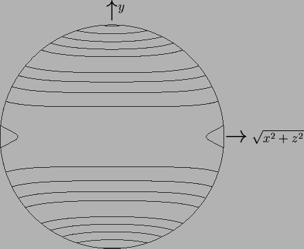
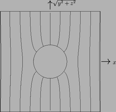
Since the stream-function is nonnegative in the lower hemisphere, $\pi/2\leq\eta\leq\pi$, the flow is radially outward along the $y$-axis and inward in the $zx$-plane, as might be expected from the distribution of vapour mass fraction and temperature given by $m_1$ and $T_1$ (fig. 8.5).

The first order correction to the flow field due to buoyancy is similar to that in a long axially heated horizontal tube (Bejan & Tien 1978). The cause is the same: the redistribution of buoyancy forces due to the primary flow leaves the lightest fluid directly above the centre of the sphere (see fig. 8.5) or tube axis. This leads to a vertical flow, which parts at the ceiling and moves outward and downward along the confining walls before returning inward along the horizontal mid-plane. The situation is the same in the lower half, but reversed.

The result of this section supports the conclusion of Mallinson and de Vahl Davis (1977) that (in the analogous pure fluid heat transfer problem) the thermal correction to the flow field depends only on the Grashof and Prandtl numbers in the combination, $\mbox{\textit{Gr}}\mbox{\textit{Pr}}=\mbox{\textit{Ra}}$.